|
Hawaii Ocean Time-series (HOT)
in the School of Ocean and Earth Science and Technology at the University of Hawai'i at Manoa |
|
| » Home » Analytical Results » Zooplankton Community Structure | ||||||||||


| ||||||||||
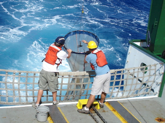
Sampling ProcedureMesozooplankton (weak swimmers 0.2-20 mm size) are collected using oblique tows of a 1-m2 net (202-µm mesh netting) from the surface to approximately 175 m depth. The catch is size fractionated by washing through a nested set of net filters and each fraction analyzed for dry weight, C and N. ResultsTemporal variation in mesozooplankton biomass during 1994-2021 is presented in Figure 64. Both zooplankton dry weight biomass (upper panel) and wet weight biomass (lower panel) are plotted. On average, zooplankton dry weight biomass was 12% of zooplankton wet weight biomass during the day (shown in red) and 13% during the night (shown in blue). The difference in biomass between zooplankton collected during the night and zooplankton collected during the day at Station ALOHA was significant for both dry and wet weights, and was caused by the upward migration of deep-living zooplankton and micronekton after sunset. | ||||||||||

